Calibration process (flatfielding and reflectance)

Introduction

Here, we process the image with flatfielding and conversion from DNs to $R^{\star}$.

In the mission, this process will be done in the ROC - but it's still useful to be able to perform calibration in PCOT on data (which could be from other cameras). Here I'm using the geology filter wheel on the training model (TRAINING_GEOLOGY).

Note that because this process uses flatfields, you need to use a PCOT camera file which contains flatfield data! You can download the appropriate file for the training model's geology wheel from the camera definition files. It's quite big!

The graph

Download graph: calibration.pcot

Figure: Flatfielding and reflectance combined. Click on image to expand.

Here's the process:

• The a/getflats(a) expr node looks at the band to filter assignments in the input image, fetches flatfield images for each band, and divides the input image by the flatfield for each band.
• The pct node locates the PCT in the image and adds regions of interest for each patch, labelled according with each patch name as it appears in the reflectance data for the PCT. It's not an automatic process, but it's not too fiddly.
• The reflectance node calculates the known reflectance in each band for each patch by combining the camera's filter response in that band by the reflectance spectrum of the patch. It then uses this this information, along with the measured reflectances (from the image) to generate gradient and intercept for the conversion to $R^\star$.
• The (a-c)/b expr node subtracts the intercept and divides by the gradient to give the calibrated image. It is important that the image input (a) should have no regions of interest, so don't take it from the pct node!

We then use a couple of multidot nodes (which create multiple circular regions of interest). These are the same, apart from the name and label colour of the regions - one was copied from the other and modified. We feed these into a spectrum so we can see how effective the calibration was.

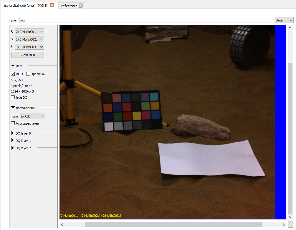
Here is the input image (taken from the input node), showing only the 670nm, 530nm and 440nm bands:

Figure: Calibration input image for RGB bands. Click on image to expand.

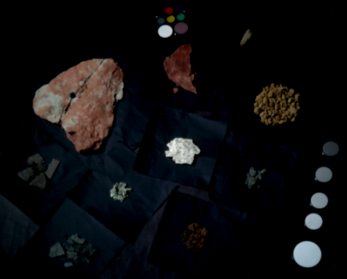
Opening the (a-c)/b node will show the calibrated result (same bands shown):

Figure: Calibration output image for RGB bands. Click on image to expand.

You'll notice that the blue cast in the original image is now mostly gone, although there the previously black background has a slight red cast (emphasised by the high gamma used for these images). That's an artifact of the non-zero intercepts in this particular calibration.

Opening the reflectance node and clicking on "Replot" will show the lines we're calibrating with. You can see that the fit is approximate because of the data, and that the intercepts are negative.

The multidot and spectrum nodes combine to show the spectra of the three brightest spectralon patches (to the right of the image) before and after calibration:

Figure: Spectra of spectralon patches before and after calibration (after is suffixed with "c"). Click on image to expand.

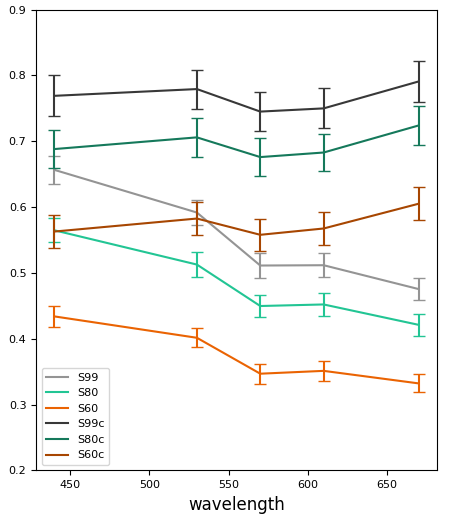
Looking at the lighter grey line (S99 before calibration) and its darker grey calibrated counterpart, we can see the result is much flatter. The same applies to the other two patches.

This is a decent result given that the lighting in this particular example image is non-uniform, and that the PCT is close to the edge.